Time-series Analysis - Part 2

In the first part of this two-part blog series about Time-Series Analysis, we have analysed time-series visually. In the second part, we will take a look at forecasting future values from the past by using Box-Jenkins Methodology. Let's dive right in:

Forecasting by Box-Jenkins methodology

The first thing we need to do before modelling is to check if our time-series is stationary. For this purpose, we can use the Augmented Dickey-Fuller Test. This test tests the hypothesis that time-series is non-stationary against the alternative that the time-series is stationary. This test is implemented in the stats models library in Python. Now we will take a look at how to use it:

from statsmodels.tsa.stattools import adfuller

dftest = adfuller(y)
dfoutput = pd.Series(dftest[0:4], 
                     index=['test statistic', 
                            'p-value', 
                            '# of lags',                             
                            '# of observations'])
print(dfoutput)

For our purpose, the p-value is the most interesting output:

test statistic        -1.365986
p-value                0.598470
# of lags             13.000000
# of observations    294.000000

As we can see from the results, the p-value is above the 0.05 critical value so we can't reject the null hypothesis that our time-series is non-stationary. With this result, we can't continue with modelling. So what are the options in a case like this? We have two easy choices: We can differentiate the time-series or we can apply a logarithm transformation (a combination of the two is also possible). Let's try the second option:

import numpy as np 

y_train_log = np.log(y_train)

By applying the Augmented Dickey-Fuller Test again on the transformed time-series we get another test result:

Results of Dickey-Fuller test:
test statistic           -3.197937
p-value                   0.020104
# of lags                13.000000
# of observations       238.000000

Finally, the p-value is below 0.05 critical value so we can reject the null hypothesis that our time-series is non-stationary. That is good news for us because on this transformed stationary time-series we can apply our forecasting models. The first approach to forecast future values is to decompose time-series and forecast each component separately. Then sum up predicted values from components at each point, to compose prediction of a time-series. We can plot this decomposition by another useful function from the statsmodels library called seasonal_decompose. The plot produced by this function is below:

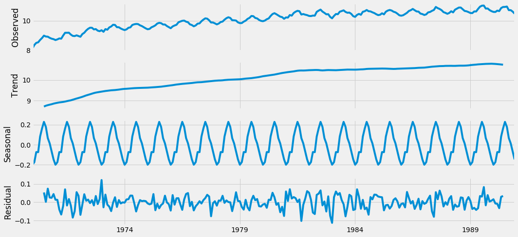
Additive decomposition of stationary time-series.

However, this approach is not generally recommended so we have to find something more appropriate. One option could be forecasting with the Box-Jenkins methodology. In this case, we will use the SARIMA (Seasonal Auto Regressive Integrated Moving Average) model. In this model, we have to find optimal values for seven parameters:

• Auto Regressive Component (p)

• Integration Component (d)

• Moving Average Component (q)

• Seasonal Auto Regressive Component (P)

• Seasonal Integration Component (D)

• Seasonal Moving Average Component (Q)

• Length of Season (s)

To set these parameters properly you need to have knowledge of auto-correlation functions and partial auto-correlation functions. One of the greatest explanations of this problem (and time-series analysis in general) I have ever read is here. In our case we have chosen SARIMA (0,1,1)x(2,0,1,12). Now it is time to fit the model to our time-series:

mdl = sm.tsa.statespace.SARIMAX(y_train_log,
                                order=(0, 1, 1),
                                seasonal_order=(2, 0, 1, 12))
                               
res = mdl.fit()

When the model is successfully fitted we are ready to try some forecasting and plot the results. We will try to forecast values from the beginning of 1991 to the end of 1995. Because we have split our data into y_train and y_test we are able to compare our predictions with real values from that time-span (our model has not seen data from y_test).

pred = res.get_prediction(start = pd.to_datetime('1991-01-01'), 
                          end = pd.to_datetime('1995-08-01'),
                          dynamic = False)

pred_ci = np.exp(pred.conf_int())
 
ax = y['1975':"1995"].plot(label = 'Observed',
                           color = '#00cedd');
np.exp(pred.predicted_mean).plot(ax = ax, 
                                 label = 'Prediction', 
                                 alpha = 0.7, 
                                 color='#ff0066');
ax.fill_between(pred_ci.index, 
                pred_ci.iloc[:, 0], 
                pred_ci.iloc[:, 1],
                color = '#ff0066',
                alpha=.25);
ax.fill_betweenx(ax.get_ylim(), 
                 pd.to_datetime('1991-01-01'), 
                 y.index[-1], 
                 alpha = 0.15,
                 zorder = -1,
                 color = 'grey');
                 
ax.set_xlabel('Date')
ax.set_ylabel('Million MJ')
plt.legend(loc = 'upper left')
plt.rcParams["figure.figsize"] = (15,7)
plt.show()

In the plot, we can see two curves, the turquoise colored curve shows real gas production values and the red curve shows the model prediction. The red area shows the confidence interval of prediction. It is clear that our model was built properly and can forecast future values with great accuracy. 

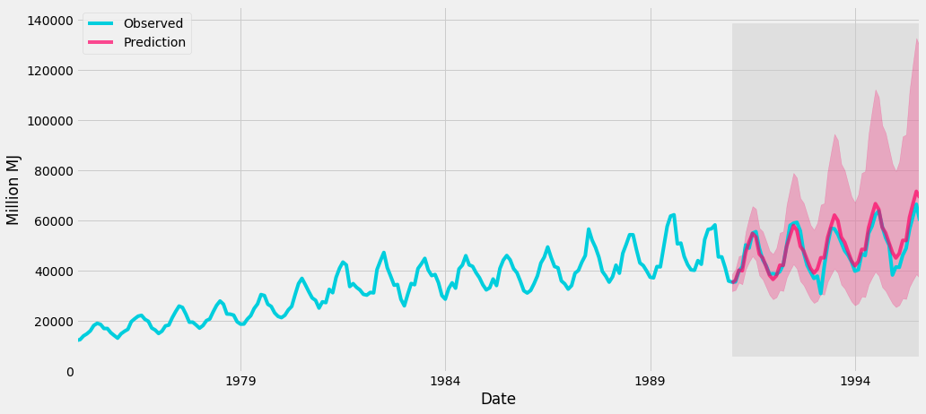
SARIMA(0,1,1)x(2,1,0,12) model prediction.

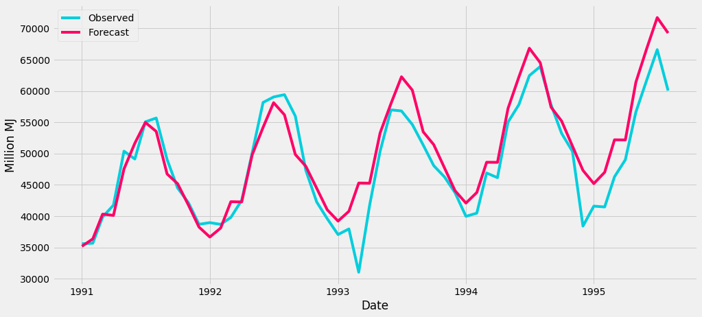
SARIMA(0,1,1)x(2,1,0,12) model prediction detail.

Conclusion

Why did we write a blog about time-series? Because we can find them in almost every business problem. Here are a few examples where time-series are taking place

• System and monitoring logs - Sysadmin and Management

• Financial/stock tickers - Finance

• Call data records - Telco

• Application clicks/surf streaming - Web/Mobile Development

• Hotels/flights reservations - Booking

• Sensor data - IOT

• and many more ...

This two-part series was just a brief introduction to Time-Series Analysis and forecasting. Data used here was chosen only for demonstrational purpose, for in actual business situations, it is much more complex to analyse time-series. If you think that Time-Series Analysis could improve your business decisions or you want to get any insights from your data, do not hesitate to contact us. 

Get in touch